Unzipping rasters in QGIS

Recently I walked the first half of the Cotswold Way (from North to South). While planning the second half, working out how many miles to attempt each day, I wanted to compare the terrain for the two halves of the walk.

The Ordnance Survey provide, as Open Data, a Digital Terrain Model (DTM) based on a 50m grid size, which is a good enough resolution for my purposes. Unfortunately the 158Mb download is for the whole of Great Britain. Another added complication is that the zip file contains a number of other zip files, one for each 10km tile. I wanted to automate the process of extracting only the necessary tiles and adding them as layers in QGIS.

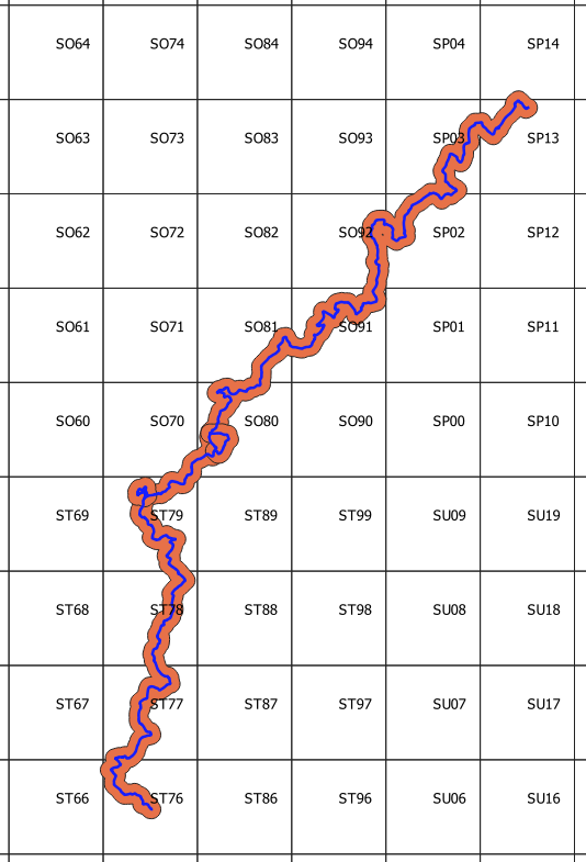
The first stage was to get the 10km grid as a QGIS layer, to determine which tiles I needed. It is possible to download all of the OS grids as a geopackage. Here the 10km grid is shown along with the route of the Cotswold Way (downloaded as a gpx file from the National trails website). I have added a 1km buffer to the route since it will be useful to also get tiles very close, but not intersecting the route (e.g. tile ST89):

Continue reading “Unzipping rasters in QGIS”

Extracting town road networks from OpenStreetMap

A while ago I worked on  a project that analysed the road networks in a number of towns and cities in England. Initially, we used the Ordnance Survey’s Integrated Transport Network (ITN). The process to extract an ITN network for a specific town was as follows:

  1. Using Digimap, extract the ITN network for a bounding box around the specific town.
  2. Extract the boundary polygon for the town and then trim the network to that polygon
  3. Tidy the road network – removing nodes (junctions) without edges (links), edges without a node at either end and disconnected islands. Fortunately, these tasks can be carried out within QGIS.

As you can imagine, this process is time-consuming and it limited the number of towns that we could analyse. Continue reading “Extracting town road networks from OpenStreetMap”

Danny Dorling and the GeoPandas

Churchyard, Cornwall

I recently picked up a copy of Danny Dorling’s So You Think You Know About Britain (Dorling, 2011) from a second-hand bookshop and it inspired me to explore some demographic data using Python and, in particular, GeoPandas.

The book discusses topics such as life expectancy, gender imbalances in the population, the concept of “optimum population”, migration, an aging population and aims to dispel the many myths that surround these matters. Continue reading “Danny Dorling and the GeoPandas”

Python, matrices, arrays, and the National Trip End Model

Travel demand in a matrix

Travel demand can be expressed using origin-destination (OD) matrices. In this example we have 4 zones:

1 2 3 4
1  10 2 9 18
2  3 2 2 1
3  2 1 15 17
4  1 3 1 4

The origins are in rows and the destinations are in columns, so number of trips from zone 1 to zone 2 is 2 and the number of trips from zone 3 to 4 is 17. Let’s say that this data is for weekday commuting trips by rail. To determine the total number of trips from zone 1 we simply sum across row 1 – 10+2+9+18=39. To determine the number of trips to zone 1 we sum down the column 10+3+2+1=16. Since the number of trips originating in zone 1 is higher than that arriving at zone 1, we can assume that zone 1 is mostly residential. Whereas we can say that zone 4 is mostly offices or factories. Continue reading “Python, matrices, arrays, and the National Trip End Model”